ICS3U JavaScript Mandelbrot Framework

Exploring the Mandelbrot Set with JavaScript

Palette. It has been said that fractal geometry is one area in which science and art meet. The software engineer generates the data; the artist's eye provides a visualization. This visualization can be most readily supplied by colour in simple systems. In more advanced systems, lighting, texture, and material properties can be added.

You are now aware that the Mandelbrot Set (M-Set) and the field around it, is really a map or collection of (integer) orbit data. These integers can be used as indicies into an array of colours (your palette). Here are some possible strategies for palette creation.

BiColor. The simplest of visualizations that does not require the creation of a palette is simply to colour points within the M-Set (orbits that do not escape) one colour (by convention: black), and another colour for those orbits that do (by convention: white).
Random. If a palette is preferred, the quickest way to create one is to populated the array with colours consisting of randomly-generated RGB values. The results are typically less than desirable as adjacent colours in the palette are unrelated, leading to unsightly banding, but the advantage is speed of development. Adding the ability to save a palette for future use would allow you to reuse the odd one that looks interesting.
Gradient. In this 'true colour', image-based world we live in, it is easy to overlook the beauty of grayscale. Ansel Adams, the 20^th Century photographer and environmentalist is best known for this stunning grayscale photographs of the American West. Creating a palette array consisting of a colour ramp extending from black to white (or any other colour bounds) is easily accomplished with a single loop.
Trigonometric. Smoother transitions between adjacent entries within a palette can be acheived through support offered by mathematical functions. Appropriately-scaled `sin` functions can easily supply smooth ramping over a range. A domain stretched over the palette size would be perfect. To summarize:
1. Define RGB colour contributions as `asin(bx+c)+d`
2. Ensure wraparound to avoid 'color borders'
3. Design for periods of integral (1..4) fractions of palette size
Examine this Excel workbook to assist with a review of the basic transformations associated with the `sin` function (if the scroll bars do not function on a Mac, you'll simply have to type in some of the data). Ensuring the period was equal to the palette size would eliminate any unsightly borders as the lower and upper values of the sine wave would connect. With the amplitude and vertical translations set to 0.5, all that would be required to create different trigonometric palettes would be to randomly generate a value for the phase shift between 0 and the size of the palette for each of the three color streams.
Enumerated. Althoguh it would be require a great deal of effort depending on the size of your palette, the precise definition of palette entries would give your project a predictable outcome.
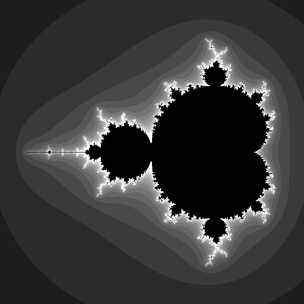
Smoothing. Despite the best attempts at palette creation noticeable banding can still occur. A blending or diffusing technique can be applied, regardless of the colouring scheme used to enhance the appeal of the image. One such strategy is referred to as the Normalized Iteration Count Algorithm (NICA). Here's a wiki on the algorithm (two-thirds of the way down under Continuous (smooth) Colouring). Here's one of the original papers on the subject. Below left is a rendering of the M-Set without the application of the NICA. The image below right shows the effect of its application. Clcik to enlarge the images.

Without NICA	With NICA

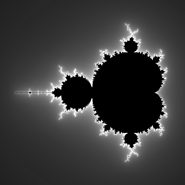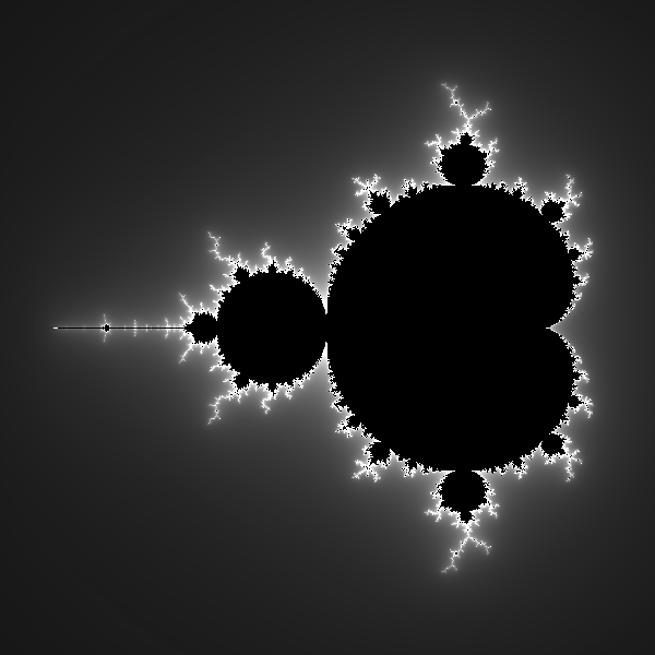
The Mandelbrot Set. The objective of this stage of the project is to render something similar to the grayscale image to the right (click to enlarge). In it, you see the Mandelbrot Set as the solid black cardioid shape in the center (with numerous bulbs or nubs attached), surrounded immediately by a white-to-black gradient extending to the edges of the square.

Here's a description of what you're seeing...

Your rendering of the Orbits in the previous stage enabled you to visualize the behaviour of `z_(i+1) larr z_i^2+c` for various `c` values. The Mandelbrot Set is simply a plot of all the pixels corresponding to `c` values that, roughly speaking, spiral inwards under the feeback loop. These pixels are rendered black. The pixels surrounding the Mandelbrot Set correspond to pixels that spiral outwards. For your first rendering, these 'field' pixels could simply be coloured, white. This would complete a B&W, bicolor image. Checking whether the orbit for a particular `c` spirals outward is easy. For each output `z_n` in the feedback loop, check its magnitude. If it's greater than 2.0, further iterations of the loop will only see the outputs grow larger. In the language of the Mandelbrot Algorithm, it is said that the orbit for this `c` value has escaped, and the corresponding pixel can be coloured white (for the time being). On the other hand, if , after a sufficient number of iterations (var orbitLength = 255), the magnitude of each `z_n` output has still not reached a magnitude of 2.0, the `c` value is considered part of the Mandelbrot Set and the corresponding pixel is coloured black.

Task.

Save your BoMShell.html as Mandelbrot.html.
Research the Mandelbrot Set and, in your own words, provide a half-panel description of either the Set of the man, accompanied by the image of Mandelbrot that appears above left (link).
An image similar to the one above right will appear in your canvas on the loading of the page. To accomplish this, you are to implement the description of algorithm provided above. Specifically, set the bounds of your real axes to [xMin,xMax] = [-2.25,0.75] and the imaginary axes to [yMin,yMax]=[-1.5,1.5]. Calculate a corresponding `Delta x` and `Delta y` value based on the canvas dimensions (they'll be equal becuase your canvas is square). From there, run a pair of nested loops over the canvas, setting the `c` value accordingly, prior to undertaking the feedback loop, checking the magnitude of each `z_n` as you go. If `|z_n|>2.0`, the loop should terminate. If it doesn't, allow a maximum of orbitLength iterations. When the loop finishes, for either reason, the pixel can be rendered in either white (if it terminated early) or black, if the orbit never 'escaped'.
Enhancement. A Zoom capability, centered on a mousedown canvas event, would be a wonderful feature to offer your viewers (just try not to spend too much time exploring the Set yourself!)

Orbits. Consider the sequence of real numbers that results from entering a positive number into your calculator and then repeatedly applying the `sqrt x` function to the previous answer. In effect, you are undertaking the feedback loop `x larr sqrt x`. As you may have guessed, this sequence of outputs tends to 1. Another interesting sequence results from the feedback loop `x larr cos x`. Be sure you're in radian mode, enter any real number, and then undertake the feedback similarly. What value or fixed point does this sequence tend towards? Does the feedback loop `x larr sin x` also tends towards a fixed point?

These feedback loops or dynamical systems are a source for interesting analysis. Benoit Mandelbrot explored the dynamical system, `z_(i+1) larr z_i^2+c` where `z_i,c in CC`. He selected a value for `c` and, starting with `z_0=0+0i`, undertook the feedback loop, generating the sequence of outputs (the orbit), `z_0, z_1, z_2,...`.

Task.

To your Orbits.html page, add the code below.

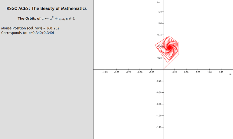
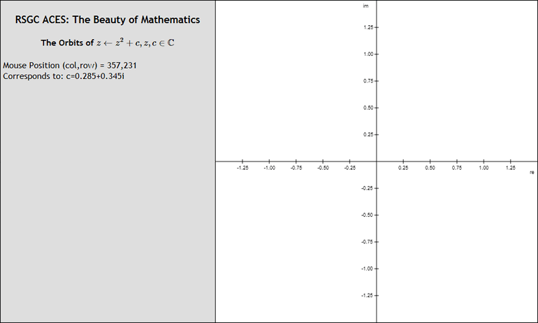
// Global variables...
...
var orbit;
var orbitLength = 255;

// Maps Re(z) to canvas column...
function canvasCol(re){
	return ...;
}

// Maps Im(z) to canvas row...
function canvasRow(im){
	return ...;
}

// draws a connected set of line segments defined by the array of Complex Numbers, o.
function drawOrbit(o){
	...
}

// populates the orbit array with the orbit of the c corresponding to MousePos
// under z<-z^2+c, in which z starts at z=0+0i
function createOrbit(mousePos){
	...
}

The purpose of this stage of the project is to offer your viewers a visualization of this dynamical system. As the mouse moves, the column and row coordinates of its hotpoint are mapped to a `c` value and the orbit (sequence of outputs) from the `z_(i+1) larr z_i^2+c` is evaluated to a length defined by orbitLength, and recorded in the array, orbit. The entire plot is then redrawn (background and axes) followed by the drawing of the orbit array as a set of connected line segments.
The path of the orbit is defined by your values for `c` and orbitLength. You may wish to limit the latter is certain situations.
Submit a thoroughly-documented Orbits.html to handin by the deadline.

Mouse-Aware Canvas. Enabling your canvas object to respond to mouse events adds significant functionality and interest to your applications. In particular, having mouse movements support our investigation of the underlying mathematics of complex numbers that defines the Mandelbrot Set will be extremely insightful. To accomplish this we need to put some familiar resources in place.

Reference: HTML5 Canvas Mouse Tutorial

Task.

Read the brief tutorial above to appreciate how an mousemove event handler is attached to your canvas object.
Copy your BoMShell.html to Orbits.html.
Duplicate the headings within the Description Panel (click to enlarge).
Add the global variables defined below and add your Axes and Plot objects from previous pages to use these values. We won't use Grid for this project, so comment out or delete references to this object. Set the tick parameter of your Axes object to 0.25. Get this stage working before continuing.
```
// Global variables...
var xMin = -1.5;
var xMax = 1.5;
var yMin = -1.5;
var yMax = 1.5;
```

Add the functions below and implement their bodies to the extent that your page duplicates the screen capture above, right. As the mouse moves, the column and row coordinates are dynamically reported to the innerHTML of a DOM element in your Description Panel, as is the corresponding complex number, `c`, that it maps to. The sequence of calls can be launched from your plot.draw() function.

// returns the column and row of the canvas that corresponds to the mouse event 
    function getMousePos(canvas, evt) {
        var rect = canvas.getBoundingClientRect();
        return {
          x: Math.floor(evt.clientX - rect.left),
          y: Math.floor(evt.clientY - rect.top)
        };
      }
      
// Maps canvas column to Re(z)
function rez(col){
	return map(...;
}

// Maps canvas row to Im(z)...
function imz(row){
	return map(...;
}

Complex Numbers. The Mandelbrot Set is based on complex numbers (a.k.a. (incorrectly) imaginary numbers - you remember these from your study of the roots of quadratic equations for which the corresponding parabolas did not have x-intercepts). In this first stage of the Mandelbrot Project you will gain familiarity with the algebra of complex numbers.

Task.

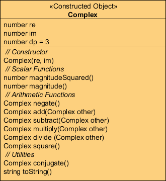
Save the file, ComplexTest.html to your javascript development folder and open it up. You'll see a reference to the script js/Complex.js. Complex.js simply offers an implementation of the UML diagram below left.
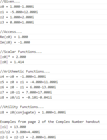
Develop and submit a documented Complex.js script (only) that, when used in conjunction with the supplied ComplexTest.html, yields the output below right.

Complex Object UML	ComplexTest Output